, 4 min read
Neural Network Training using Stiff ODE Solvers
Original post is here eklausmeier.goip.de/blog/2023/06-07-neural-networking-training-using-stiff-ode-solvers.
This post recaps the paper from Aaron J. Owens and D.L. Filkin from 1989: Efficient Training of the Back Propagation Network by Solving a System of Stiff Ordinary Differential Equations.
1. Neural network. Below is a single "neuron":
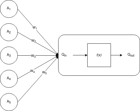
Input to node $Q$ is given in $A_i\in\mathbb{R}$, weights $W_i\in\mathbb{R}$, then node $Q$ computes
Output from node $Q$ is
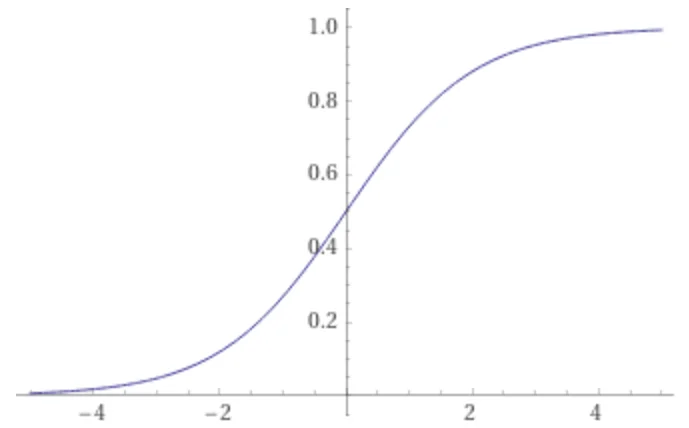
The semilinear function $f(x)$, sometimes called "squashing function", is an increasing function of $x$ that has a limited range of output values. A commonly used squashing function is the sigmoid
$\phi$ is called the threshold of the node. The squashing function has limits $0<f(x)<1$, which guarantees that the output of node $Q$ is limited to the range $0<Q_{\hbox{out}}<1$, regardless of the value $Q_{\hbox{in}}$. It looks like this, from Wolfram Alpha, for $\phi=0$.
Derivative of $f$ is
Error from output $Q_{\hbox{out}}$ versus desired output $Y$ is
Multiple "neurons" from above can be stacked together. All nodes, which are not directly connected to input or output, are called "hidden layers". Below is a three-layer neural network.
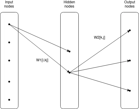
2. Gradient descent. To change the weights $W_i$ via the method of steepest descent, find the gradient of $E$ with respect to $W_i$ and then change $W_i$ to move $E$ toward smaller values. Thus change according
Applying the chain rule and using above squashing function $f$ gives
The weights are initialized to small random values. The weights are now changed according below rule:
Both $\eta$ and $\alpha$ are adjustable parameters and problem dependent. Typically with magnitudes smaller unity. Parameter $\alpha$ is called "momentum", parameter $\eta$ is called "training rate".
3. Stiff training. The authors, Owens+Filkin, were impressed by the similarities between temporal history of the weight changes and those of ordinary differential equations that are stiff. In place of the discrete equation (1), the weights $W_i$ are now to be considered functions of time. To change the weights so that the squared predition error $E$ decreases monotonically with time, the weights are required to move in the direction of gradient descent. Thus the discrete equation (1) is replaced with the ordinary differential equation (ODE)
Using the schematic equation
where $\Delta W_i$ represents the weight changes given in (2). There is one ODE for each adjustable weight $W_i$, and the right-hand sides are nonlinear functions of all weights. Comparing equations (3) and (4) shows that each unit of time $t$ in our differential equations corresponds to one presentation of the training set in the conventional algorithm, with a training rate $\eta=1$.
The Hessian matrix
is the Jacobian matrix for the differential equation. All explicit numerical solution schemes have a limiting step size for stiff stability, which is proportional to $1/\Lambda$, where $\Lambda$ is the largest eigenvalue of the Hessian matrix.
Modern stiff differential equation solvers are A-stable, so that the stability of the numerical solution is not limited by the computational stepsize taken.
The tolerance used for the numeric solver can be quite loose. Owens+Filkin chose $10^{-2}$, i.e., 1%. Owens+Filkin provide below performance table.
| RMS error | Nonstiff / stiff | gradient descent / stiff |
|---|---|---|
| 10% | 1 | 1 |
| 5% | 2 | 4 |
| 2% | 5 | >20 |
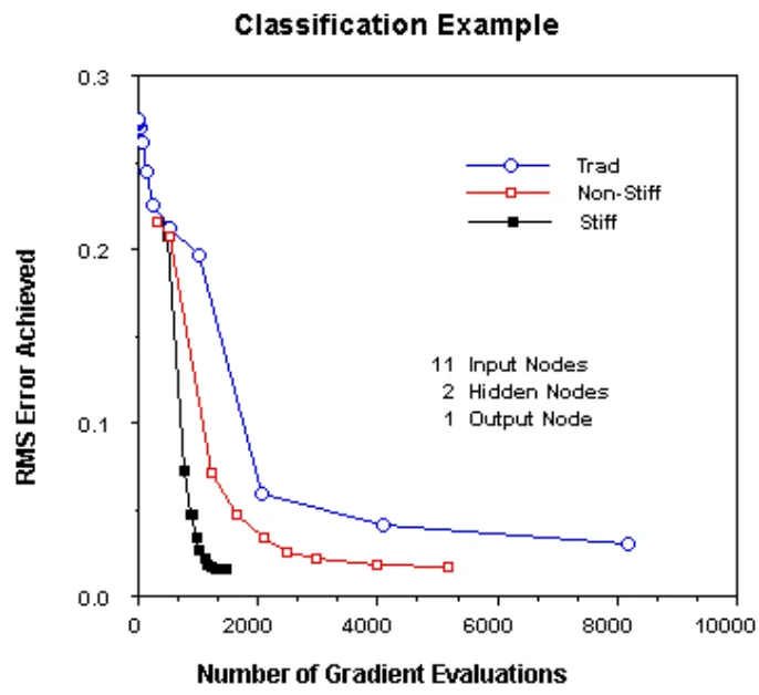
4. Classification and orientation. The results of Owens+Filkin (1989) have been confirmed by Alessio Tamburro (2019).
Fewer iterations or presentations of the data to the network are needed to reach optimal performance. [Though] The use of a ODE solver requires significantly greater computation time.
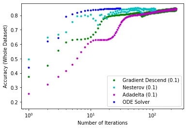
It remains remarkable that stiff ODE solvers are not used more often in the setting of neural networks. See Reply to: Neural Network Back-Propagation Revisited with Ordinary Differential Equations. The main points were:
- Tolerances employed were very strict, too strict in my opinion, especially during initial integration
- Completely incomprehensible that zvode, the "Complex-valued Variable-coefficient Ordinary Differential Equation solver" was used
- A "switching" solver, i.e., one that can automatically switch between stiff and non-stiff would likely improve the results
Currently used neural networks have quite a number of weights.
| Neural network | number of weights | reference |
|---|---|---|
| LLaMa | 13 × 109 | Wikipedia |
| ChatGPT-3 | 175 × 109 | Wikipedia |
| ChatGPT-4 | 1000 × 109 | The decoder |
Added 09-Jul-2023: Nice overview of some activation functions is here Activation Functions in Neural Networks. PyTorch's activation functions are listed here. Activation function in Twitter format as below. A separate discussion of the so called "rectifier function" is in Wikipedia. Also see Activation Functions: Sigmoid vs Tanh.
Added 07-Mar-2026: Also see Stiff-net.jl, using the Rosenbrock23 stiff ODE solver as a means for neural networks to update its weights.